Tutorial 13 — Optimisation from Python¶

Tutorial 13 of the Kalix tutorial series. You'll run the same Stringybark Creek calibration as Tutorial 12 — but driven from Python with kalix.optimise(), reading the result back as a dictionary, then simulating and plotting the calibrated model in a notebook. Expected time: about 20 minutes.

What you'll build¶

A Jupyter notebook that calibrates the Stringybark catchment model in one call, inspects the optimised parameters as a pandas object, and overlays the calibrated simulation against the observed record. This is the analysis-friendly counterpart to Tutorial 12's command-line workflow — same optimisation, same config file, driven from Python.

Prerequisites¶

Tutorial 12 complete — see Tutorial 12 — Optimisation from the commandline. We reuse its exact optimisation config and model, so the concepts (terms, statistics, parameter ranges, algorithms) carry straight over. This tutorial only changes how you launch the run.
Tutorial 5 complete — see Tutorial 5 — Running Kalix from Python. We build on the same pip install kalix package and the simulate() / pandas / matplotlib pattern you learned there.
Python 3.9 or newer with Jupyter installed.
Tutorial files — download the 013/ folder from the KalixTutorials repository. It also ships a fully-worked analysis.ipynb if you'd rather skim than type along.

Project layout¶

013/
├── data/
│   ├── climate_data.csv
│   └── observed.csv
└── models/
    ├── stringybark.ini              # the starting model
    ├── optimisation_config.ini      # the calibration recipe (same as Tutorial 12)
    └── analysis.ipynb               # the notebook we'll write

The notebook sits next to the model and config files, so the relative paths inside the config (../data/observed.csv) and the notebook resolve cleanly. Launch Jupyter from 013/models/.

The CLI and Python, side by side¶

The kalix Python package mirrors the CLI. Tutorial 12's command:

kalix optimise optimisation_config.ini stringybark.ini -s stringybark_calibrated.ini

becomes, in Python:

result = kalix.optimise(
    "optimisation_config.ini",
    model_file="stringybark.ini",
    save_model="stringybark_calibrated.ini",
)

Same three pieces — the config, the model, and where to save the calibrated model. The difference: the CLI prints a summary to the terminal, while Python returns the results to you as a dictionary you can work with directly.

Everything from Tutorial 12 — Optimisation from the commandline still applies — the [optimisation], [term.*], and [parameters] sections of the config are read exactly the same way. If you want to change the algorithm, statistic, or parameter ranges, you edit optimisation_config.ini, not the Python.

Step 1 — Open a notebook in the model folder¶

Open the 013/models folder inside your favourite Jupyter Notebook editor (e.g. VSCode or Jupyter Lab). Create a new notebook called analysis.ipynb.

Step 2 — Import Kalix and check the version¶

import kalix
import pandas as pd

print(f"kalix version: {kalix.__version__}")

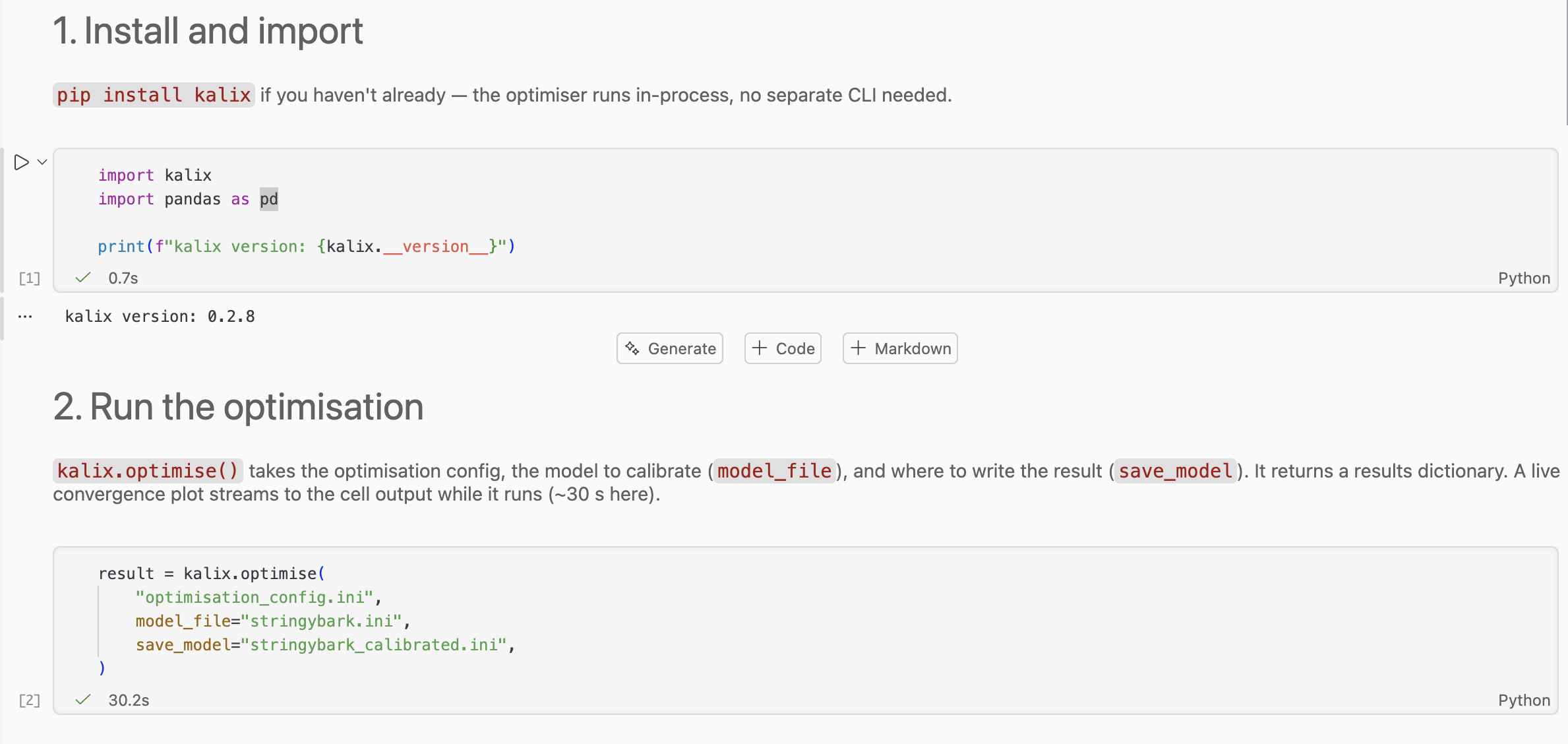
The optimiser runs in-process from the kalix package — you don't need the Kalix CLI installed separately for this tutorial.

Step 3 — Run the optimisation¶

result = kalix.optimise(
    "optimisation_config.ini",
    model_file="stringybark.ini",
    save_model="stringybark_calibrated.ini",
)

The arguments mirror the CLI:

The first positional argument is the config file.
model_file= is the model to calibrate (overrides any model_file set inside the config).
save_model= writes the calibrated model to disk. It's optional — the calibrated model also comes back inside the returned dictionary either way.

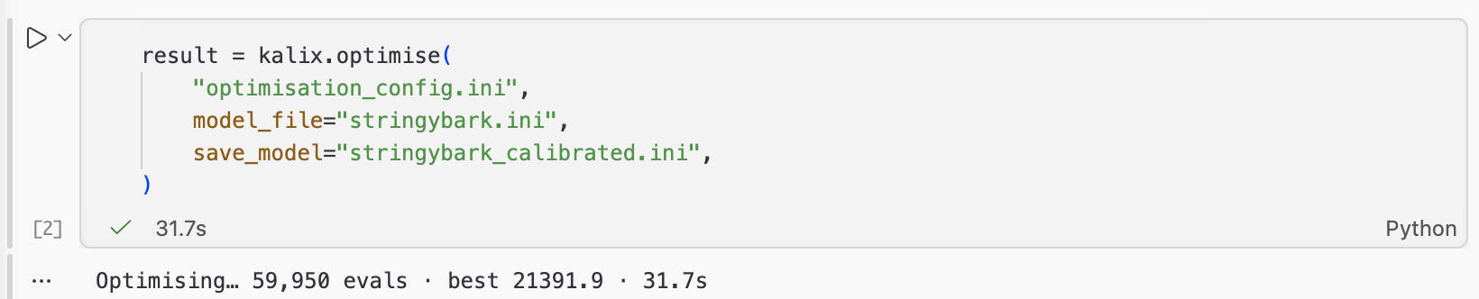
By default, kalix.optimise() prints a progress line while it runs — in a notebook it updates a single line in place (evaluations, best objective, elapsed time). The 60,000-evaluation run takes roughly 30 seconds.

If you want to handle progress callbacks yourself, pass progress=<callable> into the function. It is called once per generation with a dict (n_evaluations, best_objective, elapsed_seconds), and the built-in line is suppressed. Pass progress=False if you want to have no progress output.

Step 4 — Inspect the result¶

kalix.optimise() returns a dictionary summarising the run:

print(f"success:        {result['success']}")
print(f"message:        {result['message']}")
print(f"evaluations:    {result['n_evaluations']}")
print(f"best objective: {result['best_objective']:.3f}")

success:        True
message:        Optimisation completed successfully
evaluations:    60000
best objective: 22498.867

The full set of keys:

Key	What it holds
`best_objective`	The best objective value found (float, lower is better).
`n_evaluations`	Number of model runs performed (int).
`success`	Whether the optimiser terminated successfully (bool).
`message`	The optimiser's termination message (str).
`parameters`	The optimised parameters as a `{target: physical_value}` dict.
`optimised_model_ini`	The calibrated model serialised back to an INI string.

Differential Evolution is stochastic, so your best_objective and parameters will differ slightly from the values shown here. To make a run reproducible, add random_seed = 42 to the [optimisation] section of the config.

Step 5 — The parameters as a DataFrame¶

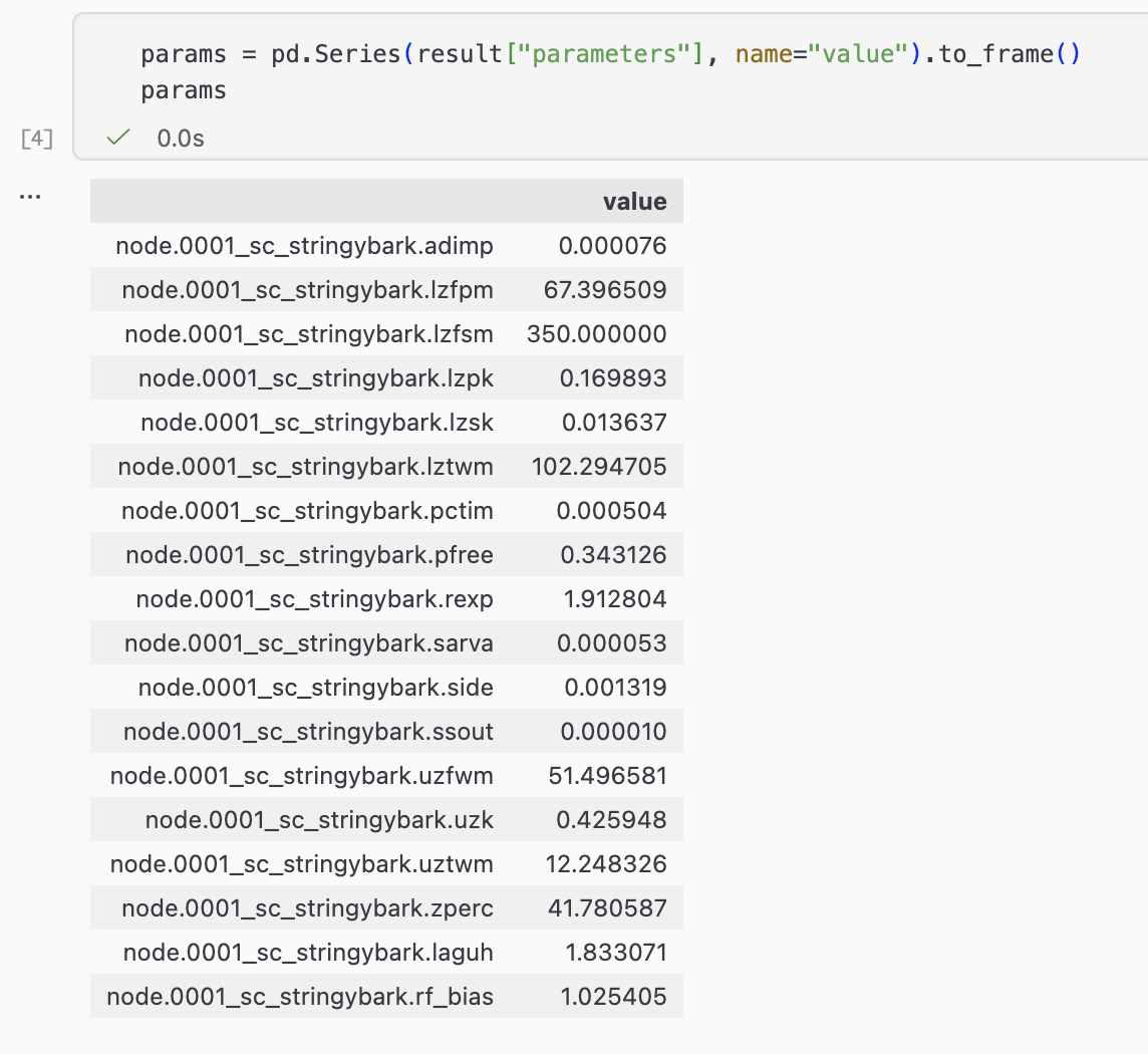
Because parameters is a plain dict, it drops straight into pandas:

params = pd.Series(result["parameters"], name="value").to_frame()
params

You'll get a tidy table of all 18 optimised values, indexed by target (e.g. node.0001_sc_stringybark.lztwm, node.0001_sc_stringybark.rf_bias). From here it's ordinary pandas — sort it, export it, or compare parameter sets across several calibrations.

Step 6 — Simulate and plot the calibrated model¶

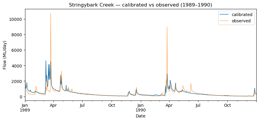
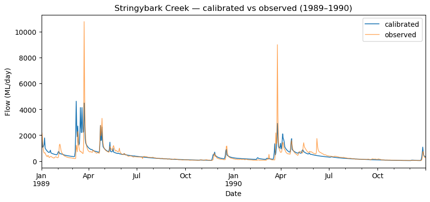
save_model= already wrote stringybark_calibrated.ini. It's an ordinary model file, so simulate it with kalix.simulate() exactly as in Tutorial 5, then overlay it against the observed record:

kalix.simulate("stringybark_calibrated.ini", output_file="calibrated_results.csv")

sim = pd.read_csv("calibrated_results.csv", parse_dates=[0], index_col=0)
obs = pd.read_csv("../data/observed.csv", parse_dates=["Date"], index_col="Date")

import matplotlib.pyplot as plt

fig, ax = plt.subplots(figsize=(10, 4))
window = slice("1989-01-01", "1990-12-31")
sim.loc[window, "node.0001_sc_stringybark.ds_1"].plot(ax=ax, label="calibrated", linewidth=1.2)
obs.loc[window, "obs"].plot(ax=ax, label="observed", alpha=0.7, linewidth=1.0)
ax.set_ylabel("Flow (ML/day)")
ax.set_title("Stringybark Creek — calibrated vs observed (1989–1990)")
ax.legend();

The calibrated simulation should track the observed hydrograph noticeably better than the starting model did.

Step 7 (bonus) — The calibrated model as a string¶

The returned dict also carries the calibrated model as INI text under optimised_model_ini — the same content save_model= wrote to disk:

print(result["optimised_model_ini"])

This is handy when you'd rather keep the calibrated model in memory — log it, diff it against the starting model, or feed it onward — without a round-trip through a file.

What to try next¶

Loop over scenarios — wrap kalix.optimise() in a loop that varies something between runs (e.g. the objective statistic, or termination_evaluations), and stack each run's parameters into a single DataFrame for comparison.
Compare statistics — point the config's statistic at ONE_MINUS_LNSE instead of SDEB, re-run, and plot both calibrated hydrographs against observed to see how the low-flow fit changes.
Make it reproducible — add random_seed = 42 to the config's [optimisation] section and confirm two runs return identical best_objective values.

Where to go from here¶

Tutorial 12 — Optimisation from the commandline — the command-line counterpart to this tutorial. CLI for batch and automation; Python for analysis — the same split you saw between Tutorials 4 and 5.

The kalix Python package lives on PyPI: pypi.org/project/kalix. Current functionality and API are documented in the package README.