Tutorial 1 — Your first model
Tutorial 1 of the Kalix tutorial series. You'll build a single-catchment rainfall-runoff model from scratch, run it, and look at the result. Expected time: about 20 minutes.
What you'll build
A daily rainfall-runoff model for the (fictional) Stringybark Creek catchment — a Sacramento catchment node feeding a downstream gauge node, driven by ~30 years of daily rainfall and PET data. By the end you'll have a working model file, a simulation, and a chart of simulated vs. observed streamflow.
Prerequisites
- Kalix software and the Tutorial files —
- Download Kalix from the Downloads page. Unzip the bundled software to a suitable place on your computer and double click “KalixIDE.exe” to launch it.
- You may want to check/set the kalix engine by following the instructions on this page: Specifying the Kalix binary path in KalixIDE.
-
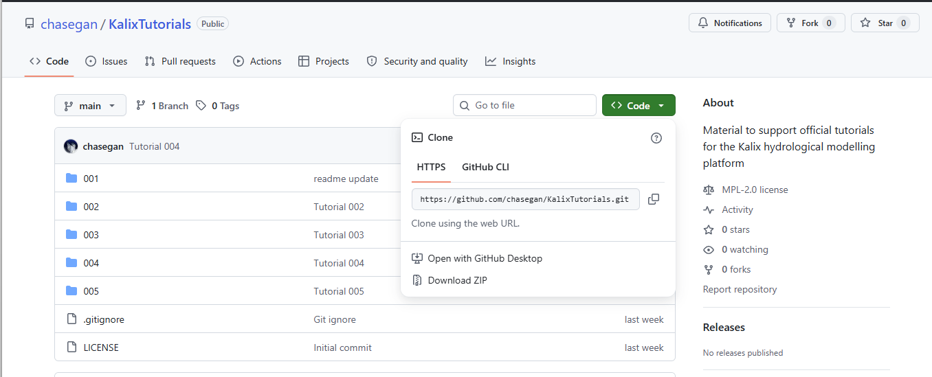
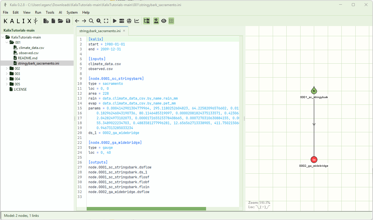
Next you will need the tutorial files. Go to the KalixTutorials repository on GitHub: https://github.com/chasegan/KalixTutorials. Click the green “Code” button and find the option that says “Download ZIP”. Unzip the tutorial material somewhere suitable. Open this folder in KalixIDE by clicking “File” > “Open Folder…”.
-
For this tutorial you will need the
001/folder. You'll need: climate_data.csv— daily rainfall and potential evaporation (mm/day)observed.csv— observed streamflow at the gauge (ML/day)- Put both CSVs in the same folder. We'll build the model file (
stringybark_sacramento.ini) from scratch in that same folder.
About the dataset
The dataset is a daily time series covering 1980-01-01 to 2009-12-31 (30 years) for a fictional catchment we'll call Stringybark Creek, with a contributing area of 228 km². Each CSV has a Date column plus one or more value columns. Here, climate_data.csv carries two value columns (rain_mm and pet_mm) while observed.csv carries one (obs).
Build the model
We'll build stringybark_sacramento.ini one section at a time. Open Kalix IDE and create a new empty model file in the same folder as the two CSVs.
Step 1 — The [kalix] section
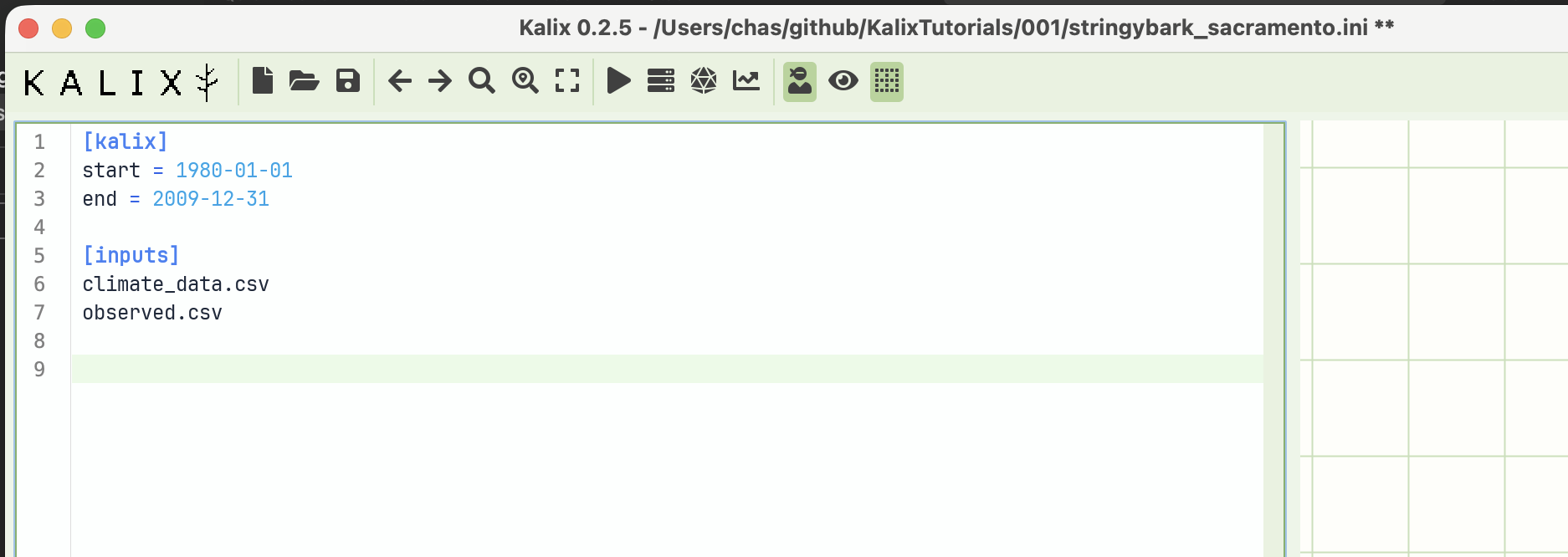
The [kalix] section holds top-level model settings. We'll use it to lock the simulation period to the 30 years our data covers.
If you leave start and end out, Kalix will infer the simulation period from the available input data. Setting them explicitly is good practice — it documents your intent and lets you simulate a sub-period without touching the data files.
Step 2 — The [data] section
The [data] section lists the data files the model will load. Bare filenames are resolved relative to the model file's folder, which is what we want here.
A single CSV can hold any number of value columns, so the count of files you list here doesn't dictate how many inputs your model can wire up. Here climate_data.csv carries both the rainfall and PET series; we'll wire each column up to the right input on the node in the next step.
Step 3 — A Sacramento catchment node
Now the heart of the model: a Sacramento rainfall-runoff node. The Sacramento Soil Moisture Accounting model takes daily rainfall and potential evaporation and produces a streamflow time series at the catchment outlet.
[node.0001_sc_stringybark]
type = sacramento
loc = 0, 0
area = 228
rain = data.climate_data_csv.by_name.rain_mm
evap = data.climate_data_alias.by_name.pet_mm
params = 0.0004142901304779964, 295.1180252604823, 64.22582096576602, 0.011943918948409236,
0.18296246043190736, 80.1146485319097, 0.00002081824375133571, 0.4230630735310133,
2.042824973102073, 0.000017265523378408665, 0.0007270310630884155, 0.00042495037393813865,
55.3489022234703, 0.4883581277996281, 12.656562713338905, 411.75021506830683,
0.9467313285033234
ds_1 = 0002_ga_widebridge
Line by line:
-
[node.0001_sc_stringybark]— declares a node with the name0001_sc_stringybark. The name is yours to choose; it's how you'll refer to this node elsewhere in the model. -
type = sacramento— picks the node type. Sacramento is one of several rainfall-runoff models Kalix supports. -
loc = 0, 0— the x,y position of this node on the IDE's network canvas. Only the IDE uses it; the simulation doesn't care. -
area = 228— catchment area in km². Sacramento outputs are scaled by area to give volumetric flow. -
rain = data.climate_data_csv.by_name.rain_mm— wires theraininput of the node to therain_mmcolumn ofclimate_data.csv. Thedata.<file>_csv.by_name.<column>syntax is how Kalix references a named column inside a loaded CSV — note how the.csvextension becomes_csvin the reference. -
evap = data.climate_data_csv.by_name.pet_mm— same idea, this time pulling thepet_mmcolumn from the same file. -
params = ...— the 17 Sacramento parameters. These were pre-calibrated for the tutorial dataset; we'll cover where they come from in the calibration tutorials. -
ds_1 = 0002_ga_widebridge— connects this node's first downstream link to a node called0002_ga_widebridge. We'll define that node in the next step; flow leaving the Sacramento node travels down this link to feed it.
As of kalix v0.3.1, input file aliases have been added, e.g.
Call on this alias by replacing the name of the file (climate_data_csv) with the alias, e.g.
Step 4 — A downstream gauge node
A gauge node is a passive node: it doesn't modify the flow passing through, it just gives you a named point in the network where the streamflow can be inspected and recorded. Real-world gauges are physical streamflow measurement stations; gauge nodes are the modelling equivalent.
Line by line:
-
[node.0002_ga_widebridge]— declares the gauge node. This is the node referenced byds_1on the Sacramento node above. -
type = gauge— picks the node type. Flow passes through unchanged. -
loc = 0, 40— positions the node below the Sacramento node on the IDE's canvas.
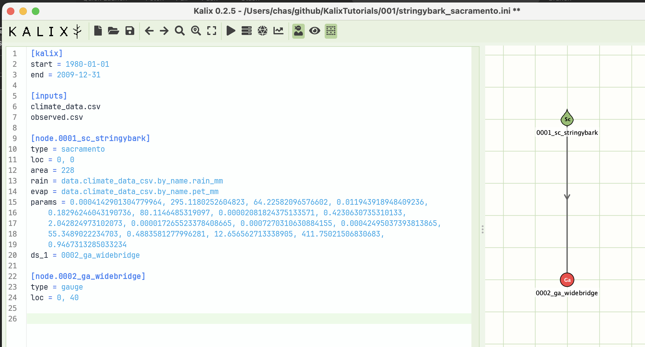
Step 5 — The [outputs] section
The [outputs] section lists the model results we want to record. We'll record flow at both nodes plus the three Sacramento runoff components.
[outputs]
node.0001_sc_stringybark.dsflow
node.0001_sc_stringybark.ds_1
node.0001_sc_stringybark.flosf
node.0001_sc_stringybark.flobf
node.0001_sc_stringybark.floin
node.0002_ga_widebridge.dsflow
These are:
-
node.0001_sc_stringybark.dsflow— total downstream flow leaving the Sacramento node (ML/day). -
node.0001_sc_stringybark.ds_1— the flow going down the first downstream link, i.e. the link feeding the gauge. With only one downstream connection here, this matchesdsflow. -
node.0001_sc_stringybark.flosf— surface runoff component (overland flow). -
node.0001_sc_stringybark.flobf— baseflow component (slow-release groundwater). -
node.0001_sc_stringybark.floin— interflow component (shallow subsurface flow). -
node.0002_ga_widebridge.dsflow— flow leaving the gauge node. Since gauges don't modify flow, this should equal the inflow it receives from upstream.
The Sacramento dsflow is the sum of the three runoff components (flosf + flobf + floin).
The finished model file
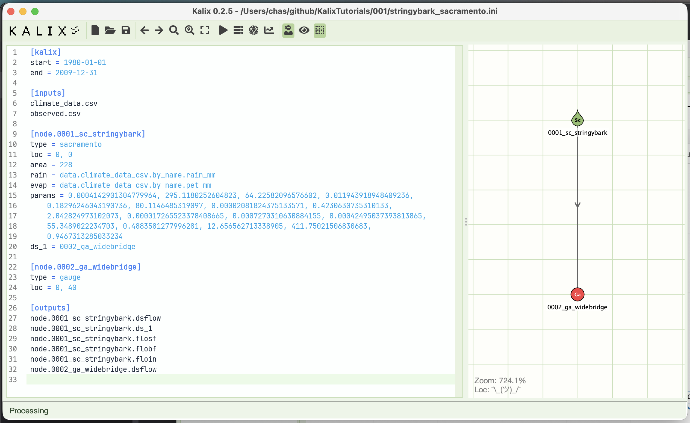
Putting it all together, stringybark_sacramento.ini should look like this:
[kalix]
start = 1980-01-01
end = 2009-12-31
[data]
climate_data.csv
observed.csv
[node.0001_sc_stringybark]
type = sacramento
loc = 0, 0
area = 228
rain = data.climate_data_csv.by_name.rain_mm
evap = data.climate_data_csv.by_name.pet_mm
params = 0.0004142901304779964, 295.1180252604823, 64.22582096576602, 0.011943918948409236,
0.18296246043190736, 80.1146485319097, 0.00002081824375133571, 0.4230630735310133,
2.042824973102073, 0.000017265523378408665, 0.0007270310630884155, 0.00042495037393813865,
55.3489022234703, 0.4883581277996281, 12.656562713338905, 411.75021506830683,
0.9467313285033234
ds_1 = 0002_ga_widebridge
[node.0002_ga_widebridge]
type = gauge
loc = 0, 40
[outputs]
node.0001_sc_stringybark.dsflow
node.0001_sc_stringybark.ds_1
node.0001_sc_stringybark.flosf
node.0001_sc_stringybark.flobf
node.0001_sc_stringybark.floin
node.0002_ga_widebridge.dsflow
Run it
Save the file. Hit the Run button in Kalix IDE (or use the Run menu).
The simulation should finish in a fraction of a second.
Look at the output
The Run Manager window should open to a blank chart view. In order to plot node.0002_ga_widebridge.dsflow against the obs column of observed.csv, we must first load the data into the Run Manager. To load observed.csv, click and drag it from either your system file explorer or the KalixIDE file tree into the run manager window:
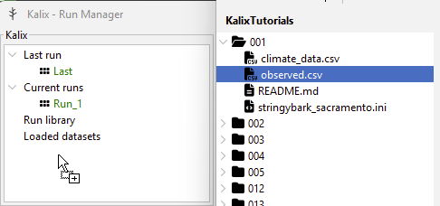
Once loaded, verify that it appears in the “Loaded datasets” dropdown menu. Next, click the “Last” run icon, hold Ctrl/Cmd to select multiple data sources, and then click observed.csv under “Loaded datasets”. Your Kalix and Timeseries panes should look like this:
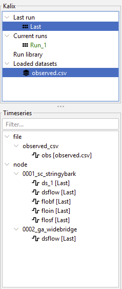
You can now click the outputs (hold Ctrl/Cmd to select multiple timeseries) to plot node.0002_ga_widebridge.dsflow against the obs column of observed.csv. The Widebridge gauge sits at the catchment outlet, so its flow record is what you'd compare against the observed gauge data.
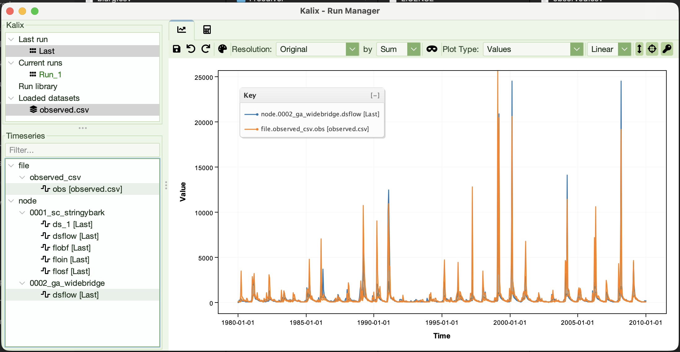
Try zooming and manipulating the plot window. A few specific interactions to try:
-
Hold shift and drag to zoom in on a window.
-
Double click to reset the zoom window.
-
Try the controls along the top of the graph, particularly the three buttons on the right.
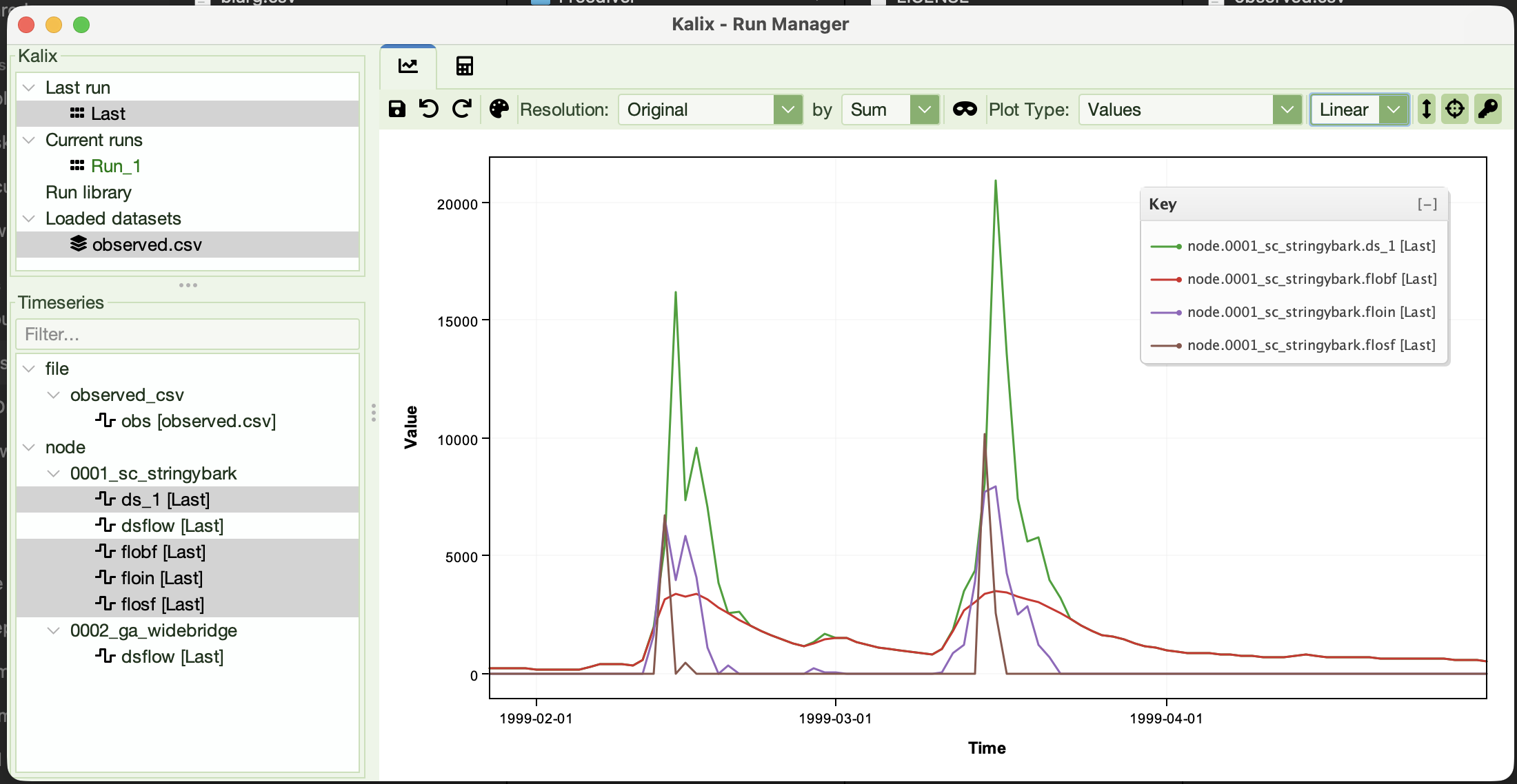
Try also plotting the three Sacramento flow components (flosf, flobf, floin) together. You'll see that:
-
baseflow (
flobf) is the steady background contribution -
surface flow (
flosf) is the spiky response to storms -
interflow (
floin) sits in between, draining off after wet periods
What to try next
Small experiments to build intuition. Change one thing at a time and re-run.
-
Change the catchment area — set
area = 114(half of the original value) and observe hownode.0001_sc_stringybark.dsflowscales. Note: You can click multiple runs to compare the flow volumes on the same plot. -
Change the simulation period — set
start = 2000-01-01to run only the last 10 years. Useful when you're iterating on parameters and want fast feedback. -
Tweak a parameter — the 6th parameter (
80.1146…) is Sacramento's lower-zone tension water capacity. Halve it and re-run; the catchment should saturate more easily and respond faster to rainfall. -
Inspect the link — add
node.0002_ga_widebridge.usflowto the outputs to record the flow arriving at the gauge from upstream. Plot it alongsidenode.0001_sc_stringybark.dsflow— the two series should overlay exactly, since the link between them doesn't modify flow.
Where to go from here
Once you're comfortable with this two-node setup, the next tutorials cover the rest of the foundations before we tackle bigger models:
-
Tutorial 2 — Expressions — apply mathematical expressions to your inputs (using rainfall as the example) and compare runs with the Run Manager's plotting tools.
-
Tutorial 3 — Relative paths and trailhead paths — organise input data with portable path references that survive moving the model around.
-
Tutorial 4 — Running Kalix from the commandline — drive Kalix from the CLI instead of the IDE.