Tutorial 12 — Optimisation from the commandline¶

Tutorial 12 of the Kalix tutorial series. You'll calibrate the Stringybark Creek model from a terminal using kalix optimise — reading an optimisation config file, watching the live convergence plot, and saving a calibrated model ready to run. Expected time: about 20 minutes.

What you'll build¶

A working command-line calibration of the Stringybark catchment model. You'll point kalix optimise at an optimisation config file and a model file, let the Differential Evolution optimiser tune 18 parameters against an observed flow record, watch it converge in the terminal, and write out a calibrated model file ready to simulate.

Prerequisites¶

Optimisation in the GUI — you should already have run a calibration inside Kalix IDE (covered in an earlier optimisation tutorial — [mention-page placeholder once that tutorial is published]). This tutorial assumes you understand the basic idea: parameters, an objective statistic, and an observed series to fit against. Here we just move that same workflow to the command line.
Tutorial 4 complete — see Tutorial 4 — Running Kalix from the commandline. We reuse the kalix CLI and the same project conventions (trailhead paths, kalix sim).
Kalix CLI installed — see Downloads. Verify with kalix --version from a fresh terminal.
Tutorial files — download the 012/ folder from the KalixTutorials repository.

Project layout¶

012/
├── data/
│   ├── climate_data.csv             # rain_mm + pet_mm
│   └── observed.csv                 # obs — the streamflow we calibrate against
└── models/
    ├── stringybark.ini              # the starting model
    ├── optimisation_config.ini      # the calibration recipe
    └── stringybark_calibrated.ini   # the result (we'll regenerate this)

The model uses trailhead paths (^/data/...), so it runs from any depth — exactly as you set up in Tutorial 3. All commands below assume you've changed into 012/models/.

The two ingredients¶

Calibration on the command line needs two files:

The model file (stringybark.ini) — the thing being calibrated. It's an ordinary Kalix model with starting parameter values. The optimiser overwrites the parameters listed in the config and leaves everything else untouched.
The optimisation config (optimisation_config.ini) — the recipe: which parameters to tune, over what ranges, against which observed data, using which objective and algorithm.

This mirrors kalix simulate from Tutorial 4, which took a single model file. kalix optimise takes the config and the model.

Anatomy of the optimisation config¶

Open optimisation_config.ini. It has three parts.

The `[optimisation]` section — the algorithm¶

[optimisation]
objective_expression = term1
algorithm = DE
de_cr = 0.9
population_size = 50
de_f = 0.8
termination_evaluations = 60000
n_threads = 12

Line by line:

objective_expression = term1 — the quantity to minimise. It refers to a term defined below. It's an expression, so you can combine several terms — e.g. 0.5*term1 + 0.5*term2 — for multi-objective calibration.
algorithm = DE — the search algorithm. Kalix supports several including DE (Differential Evolution), CMAES (CMA-ES), and SCE (Shuffled Complex Evolution).
de_cr = 0.9, de_f = 0.8 — DE's crossover rate and differential weight. The defaults (0.9 and 0.8) are sensible; leave them unless you know you want to change them.
population_size = 50 — number of candidate parameter sets DE maintains each generation.
termination_evaluations = 60000 — stop after this many model runs. More evaluations means a more thorough search but a longer run.
n_threads = 12 — evaluate candidates in parallel across this many threads. Set it near your CPU's core count.

The `[term.term1]` section — the objective¶

[term.term1]
simulated = node.0001_sc_stringybark.ds_1
observed_file = ../data/observed.csv
observed_series = 1
statistic = SDEB

A term pairs a simulated series with an observed one and scores the fit:

simulated = node.0001_sc_stringybark.ds_1 — the model output to compare. This is the same series you'd list under [outputs] to record (and indeed stringybark.ini records exactly this).
observed_file = ../data/observed.csv — the observed data, as a relative path from the config folder.
observed_series = 1 — which value column to use. It's a 1-based index over the value columns (the date column doesn't count), so 1 is the obs column. You can also name it directly: observed_series = obs.
statistic = SDEB — the goodness-of-fit measure. Every Kalix statistic is framed so that lower is better and 0 is perfect. Available options:

Name	Meaning
`SDEB`	Sorted Data Error with Bias — blends timing error, flow-distribution error, and a bias penalty. A good general-purpose default.
`ONE_MINUS_NSE`	1 − Nash–Sutcliffe Efficiency.
`ONE_MINUS_LNSE`	1 − log-NSE. Emphasises low flows.
`ONE_MINUS_KGE`	1 − Kling–Gupta Efficiency.
`ONE_MINUS_PEARS_R`	1 − Pearson correlation.
`RMSE`	Root mean square error.
`MAE`	Mean absolute error.
`ABS_PBIAS`	Absolute percent bias.

The `[parameters]` section — what to tune¶

[parameters]
node.0001_sc_stringybark.adimp = log_range(g(1),1E-05,0.15)
node.0001_sc_stringybark.lzfpm = log_range(g(2),1,300)
...
node.0001_sc_stringybark.laguh = lin_range(g(17),0,3)
node.0001_sc_stringybark.rf_bias = lin_range(g(18),0.7,1.3)

Each line maps a model property to a search range driven by a gene g(n):

The left side is the address of the parameter to optimise — the same dotted path you'd use anywhere else in Kalix. Here we tune the 17 Sacramento parameters plus rf_bias, a rainfall bias-correction factor on the node. (rf_bias shows up in the saved model as the leading multiplier on the rain = expression — the link back to the expressions you wrote in Tutorial 2.)
g(n) is the n-th optimisation variable: a normalised value in [0, 1] that the algorithm searches. Each gene is used once.
log_range(g(n), min, max) searches logarithmically between min and max — right for parameters spanning orders of magnitude, like storage capacities and rate constants.
lin_range(g(n), min, max) searches linearly — right for parameters with a natural additive scale, like laguh (lag, 0–3 days) and rf_bias (0.7–1.3).

For the full optimisation-config reference (every key, every statistic and algorithm), see the optimisation reference — [mention-page placeholder].

Step 1 — Verify the command¶

From 012/models/, check the subcommand and its flags:

kalix help optimise

Run parameter optimisation

Usage: kalix optimise [OPTIONS] <CONFIG_FILE> [MODEL_FILE]

Arguments:
  <CONFIG_FILE>  Path to the optimisation configuration file (.ini)
  [MODEL_FILE]   Path to the model file (.ini). Overrides model_file in config if specified

Options:
  -s, --save-model <SAVE_MODEL>     Path to save the optimised model file (.ini)
  -q, --quiet                       Suppress terminal output and plotting
  -r, --report-frequency <N>        Plot updates every N evaluations [default: 20]
  -p, --profile                     Report execution time profile
  -h, --help                        Print help

Step 2 — Run the optimisation¶

kalix optimise optimisation_config.ini stringybark.ini -s stringybark_calibrated.ini

The three arguments:

optimisation_config.ini — the config (the recipe).
stringybark.ini — the model to calibrate.
-s stringybark_calibrated.ini — where to write the calibrated model. Without -s, the optimiser still runs and reports results, but writes no file.

Kalix first echoes back what it parsed, so you can sanity-check the setup before the search starts:

Loading optimisation configuration: optimisation_config.ini
Objective expression: term1
Terms (1):
  term1 = SDEB(node series 'node.0001_sc_stringybark.ds_1', obs '../data/observed.csv')
Algorithm: DE
Population size: 50
Termination evaluations: 60000
Number of parameters: 18
Loading model: stringybark.ini
Term 'term1': loaded 10958 observed points from ../data/observed.csv

=== Starting Optimisation ===

Step 3 — Watch it converge¶

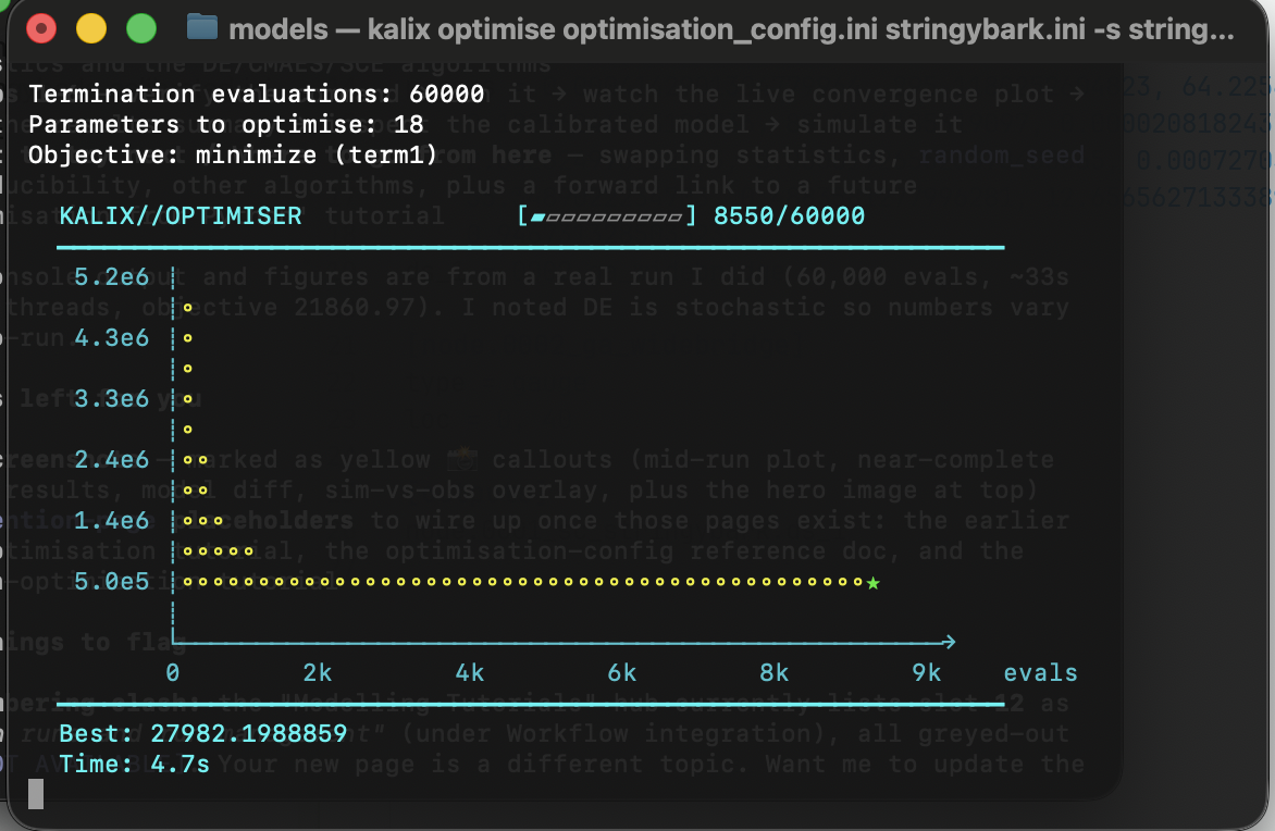
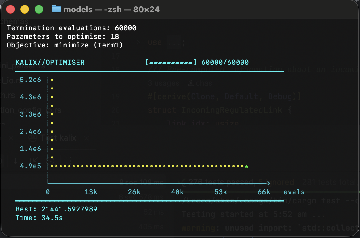
As it runs, Kalix draws a live convergence plot right in the terminal — best objective value (vertical axis) against evaluations (horizontal axis), with a progress bar and a running best score. You'll watch the curve drop steeply at first, then flatten as the search homes in.

The whole 60,000-evaluation run finishes in roughly 30 seconds on a 12-thread machine — each model run is only a few milliseconds, and n_threads evaluates many in parallel. Prefer a clean run with no plotting (e.g. for logging)? Add -q.

Step 4 — Read the results summary¶

When it finishes, Kalix prints a summary: the final objective value, the optimised genes (normalised [0,1]), and the same parameters as physical values — the numbers that actually go into the model.

=== Optimisation Complete ===
Status: SUCCESS
Message: Optimisation completed successfully
Function evaluations: 60000
Best objective value: 21860.969497

Optimized Parameters (physical values):
  node.0001_sc_stringybark.adimp = 0.023690
  node.0001_sc_stringybark.lzfpm = 73.962576
  ...
  node.0001_sc_stringybark.laguh = 1.847684
  node.0001_sc_stringybark.rf_bias = 1.024898

Optimized model written to: stringybark_calibrated.ini
Done!

Differential Evolution is stochastic, so your exact numbers will differ slightly from run to run (and from the file shipped in the repo). To make a run reproducible, add random_seed = 42 to the [optimisation] section.

A quick read of the physical values is a useful gut-check: are any parameters pinned right at the edge of their log_range/lin_range bounds? If so, that bound may be too tight — widen it in the config and re-run.

Step 5 — Inspect the calibrated model¶

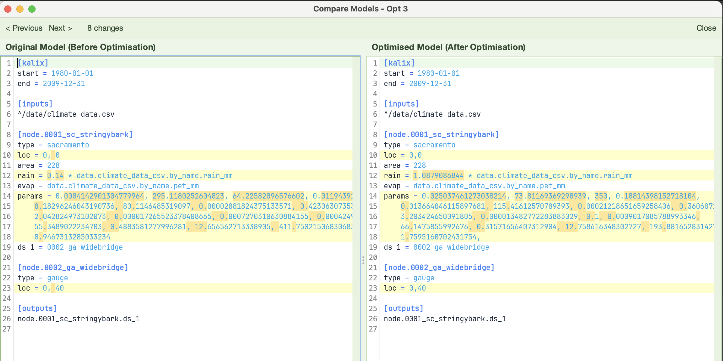
Open stringybark_calibrated.ini. It's a complete, runnable model — identical to stringybark.ini except for the tuned parameters:

The params = ... line now holds the optimised Sacramento values.
The rain = ... line's leading multiplier has changed from the starting value to the calibrated rf_bias, e.g. rain = 1.024898 * data.climate_data_csv.by_name.rain_mm.

Step 6 — Simulate the calibrated model¶

The calibrated file is just a model, so run it the way you ran models in Tutorial 4:

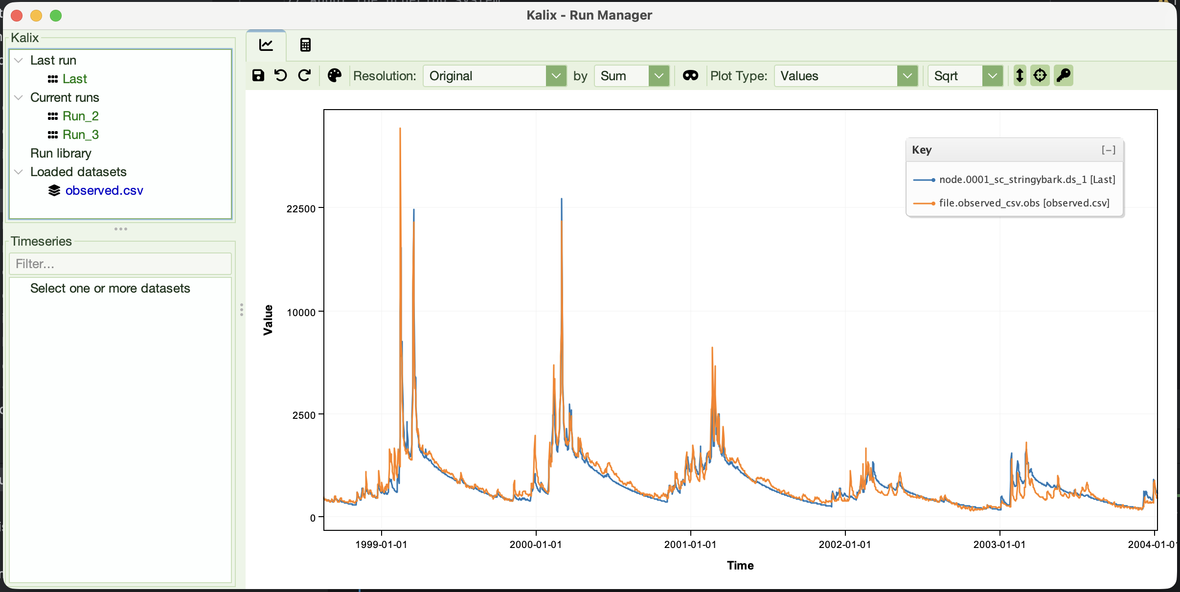
kalix sim stringybark_calibrated.ini -o calibrated_results.csv

Load calibrated_results.csv and ../data/observed.csv and overlay them (in the IDE, the Run Manager, or pandas as in Tutorial 5). The calibrated simulation should track the observed hydrograph noticeably better than the starting model did.

What to try next¶

Change one thing at a time and re-run.

Swap the objective statistic — change statistic = SDEB to ONE_MINUS_LNSE and re-run. Log-NSE rewards low-flow fit; compare the recession limbs against the SDEB calibration.
Make it reproducible — add random_seed = 42 to [optimisation], run twice, and confirm you get identical results.
Trade runtime for thoroughness — drop termination_evaluations to 10000 for a quick-and-rough fit, or raise it to 120000 for a more exhaustive search. Watch the convergence plot to judge whether more evaluations are still buying improvement.
Try another algorithm — switch algorithm = DE to algorithm = SCE (add complexes = 5) or algorithm = CMAES (add sigma = 0.3). Compare final objective values and convergence behaviour.
Hold parameters fixed — if you trust some parameters, remove their lines from [parameters] so the optimiser focuses on the rest.

Where to go from here¶

Optimisation from Python — the same calibration driven from a notebook via the kalix package, so you can script multi-site calibrations and post-process the results in pandas. CLI for batch and automation; Python for analysis — the same split you saw between Tutorial 4 — Running Kalix from the commandline and Tutorial 5 — Running Kalix from Python. [mention-page placeholder once the Python optimisation tutorial is published]

For the full CLI reference (every command, every flag), see Commandline.