Tutorial 2 — Expressions
Tutorial 2 of the Kalix tutorial series. You'll take the model from Tutorial 1 and rewrite its rainfall input as a weighted combination of three gauge stations, then compare runs side-by-side in the Run Manager. Expected time: about 15 minutes.
What you'll build
The same Stringybark Creek catchment from Tutorial 1, but with the rainfall input rebuilt from three rain gauge stations instead of a single areal-rainfall series. The new rain is constructed inside the model file using a Kalix expression — a piece of arithmetic that combines data references and literal numbers.
Prerequisites
-
Kalix software and the Tutorial files — refer to Tutorial 1 — Your first model.
-
Tutorial 1 complete — refer to Tutorial 1 — Your first model.
-
Tutorial files — download the
002/folder from the KalixTutorials repository. You'll need: rain_north.csv,rain_central.csv,rain_south.csv— daily rainfall at three stations around the catchment (mm/day)climate_data.csv— same file as Tutorial 1; we'll only use thepet_mmcolumn this timeobserved.csv— same as Tutorial 1
Put all five CSVs in the same folder. We'll build the new model file (stringybark_expressions.ini) alongside them.
About expressions
In Tutorial 1 you wrote rain = data.climate_data_csv.by_name.rain_mm — a direct reference to a single column. But that = is more powerful than it looks. Most node properties that accept data actually accept a mathematical expression rather than just a simple data reference.
The expression language is rich. It includes:
-
Data references —
data.<file>_csv.by_name.<column>, exactly as in Tutorial 1 -
Numeric literals — plain numbers like
0.5,1.1,3.14 -
Arithmetic operators —
+,-,*,/,^(power), with parentheses for grouping -
Conditional logic —
if(condition, true_value, false_value)with comparison operators (<,>,==, …) -
Common math functions —
max,min,abs,sqrt,pow,log,sin,floor, and many more -
Model result references — feed one node's output into another node's input
-
Simulation context variables — the
sim.*namespace exposes the current simulation date (sim.year,sim.month,sim.day, …), useful for time-of-year switching
A few quick examples to make this concrete:
-
rain = 1.1 * data.climate_data_csv.by_name.rain_mm— scale rainfall up by 10% to simulate a wetter climate scenario. -
evap = data.climate_data_csv.by_name.pet_mm * 0.95— apply a 5% PET reduction. -
inflow = 2.5 * data.upstream_csv.by_name.flow— on aninflownode (a node type that injects flow at a point in the network), scale an upstream inflow series by 2.5×.
This tutorial focuses on the most common case — building a single rainfall input from multiple gauges.
For the full expression language reference, see Dynamic Expressions.
Build the model
Open Kalix IDE and create a new model file called stringybark_expressions.ini in the same folder as the five CSVs. The fastest way is to copy your Tutorial 1 model file (stringybark_sacramento.ini) and rename the copy. The structure is identical except for two small changes below.
Step 1 — Add the three station files to [data]
We've kept climate_data.csv so we can still pull pet_mm from it, and we've added the three new station files. The rain_mm column inside climate_data.csv is still loaded but we're about to stop referencing it.
Step 2 — Replace the rain line with a weighted expression
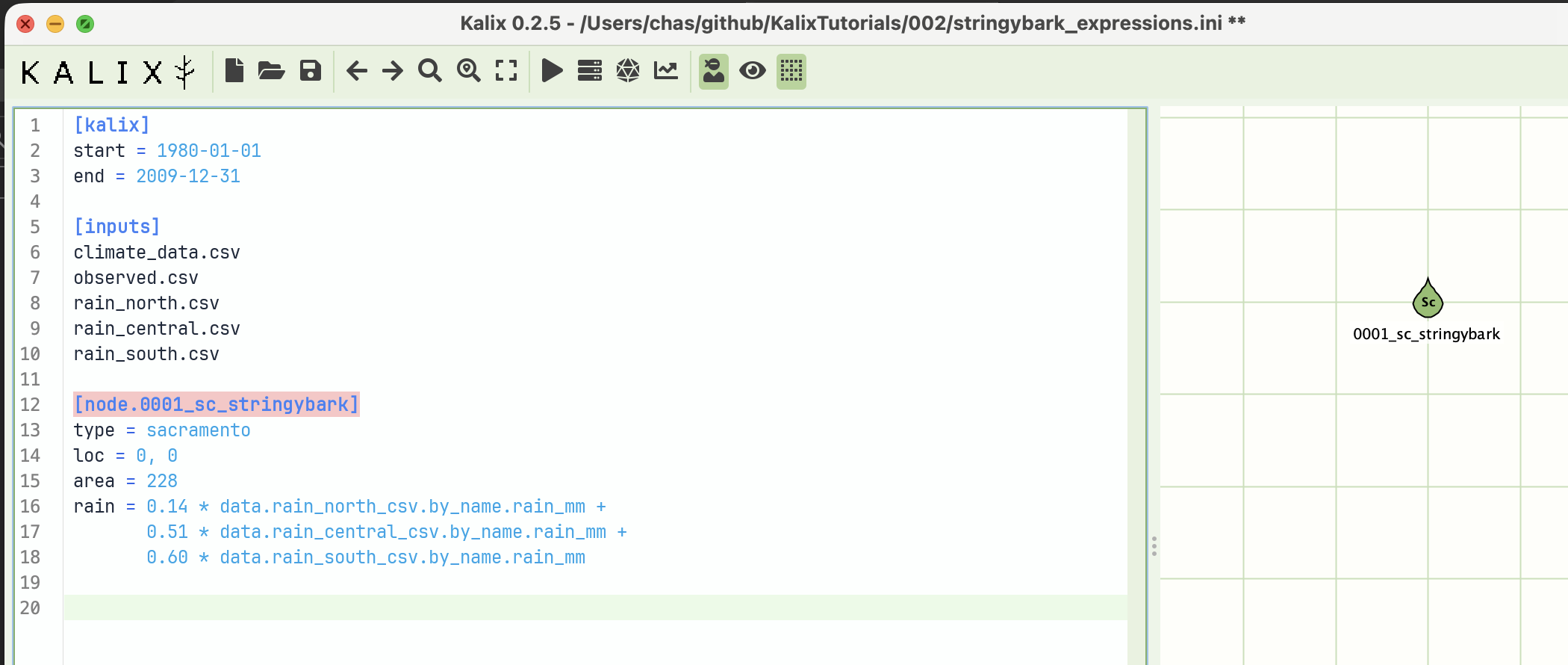
In the Sacramento node, replace the old single-source rain line with this:
rain = 0.14 * data.rain_north_csv.by_name.rain_mm +
0.51 * data.rain_central_csv.by_name.rain_mm +
0.60 * data.rain_south_csv.by_name.rain_mm
What's happening:
-
Three data references, one for each station, each pulling the
rain_mmcolumn. -
Each is multiplied by a numeric weight reflecting that station's relative contribution to the catchment's areal rainfall (think Thiessen-polygon weights).
-
The products are summed with
+to give the final rainfall driving the Sacramento model. -
The expression spans three lines for readability — Kalix joins any line beginning with whitespace onto the previous line, so the leading indent isn't just for looks; it's what tells the parser these three lines are one expression. The trailing
+operators don't matter for continuation; they're just part of the arithmetic.
Note the weights don't need to sum to 1 — they're whatever you decide reflects each station's contribution. Here the sum (~1.25) means the combined rainfall is a bit heavier than any individual station, which is what you'd expect when stations cover overlapping parts of the catchment.
The finished model file
The rest of the file is unchanged from Tutorial 1. Putting it all together:
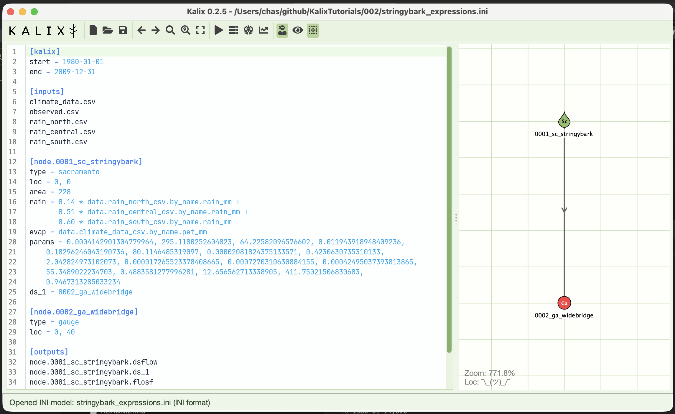
[kalix]
start = 1980-01-01
end = 2009-12-31
[data]
climate_data.csv
observed.csv
rain_north.csv
rain_central.csv
rain_south.csv
[node.0001_sc_stringybark]
type = sacramento
loc = 0, 0
area = 228
rain = 0.14 * data.rain_north_csv.by_name.rain_mm +
       0.51 * data.rain_central_csv.by_name.rain_mm +
       0.60 * data.rain_south_csv.by_name.rain_mm
evap = data.climate_data_csv.by_name.pet_mm
params = 0.0004142901304779964, 295.1180252604823, 64.22582096576602, 0.011943918948409236,
0.18296246043190736, 80.1146485319097, 0.00002081824375133571, 0.4230630735310133,
2.042824973102073, 0.000017265523378408665, 0.0007270310630884155, 0.00042495037393813865,
55.3489022234703, 0.4883581277996281, 12.656562713338905, 411.75021506830683,
0.9467313285033234
ds_1 = 0002_ga_widebridge
[node.0002_ga_widebridge]
type = gauge
loc = 0, 40
[outputs]
node.0001_sc_stringybark.dsflow
node.0001_sc_stringybark.ds_1
node.0001_sc_stringybark.flosf
node.0001_sc_stringybark.flobf
node.0001_sc_stringybark.floin
node.0002_ga_widebridge.dsflow
Run it
Save the file. Hit the Run button in Kalix IDE.
Compare with Tutorial 1 in the Run Manager
Run both the Tutorial 1 and Tutorial 2 models in Kalix IDE, and open the Run Manager. Select both runs and use the Run Manager's plotting tool to overlay node.0002_ga_widebridge.ds_1 from each. You should see two streamflow series that are visibly similar but not identical — the new rainfall (a weighted blend of three station series) produces a slightly different streamflow than the single areal-rainfall series in Tutorial 1.
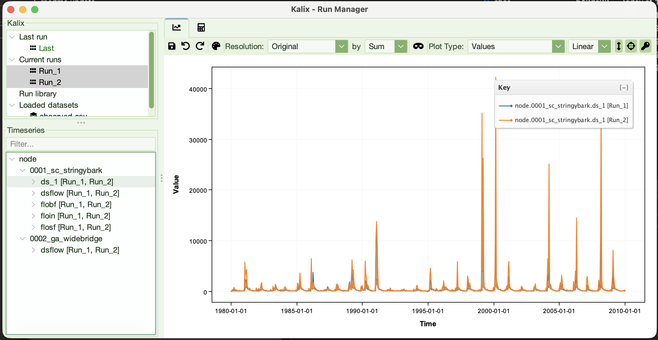
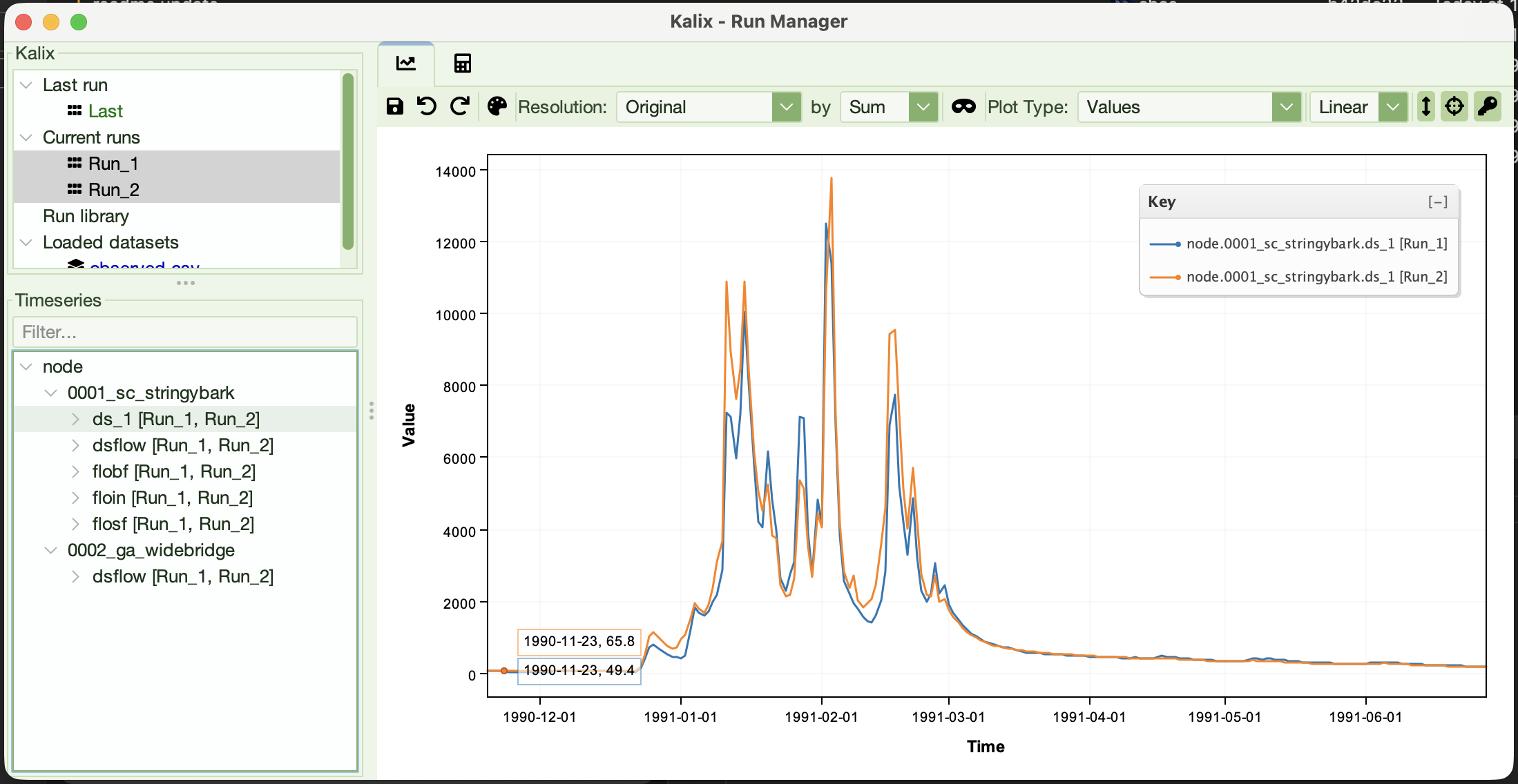
Look at the overlay carefully. You'll likely see:
-
Storm peaks shifted slightly in magnitude
-
Recession limbs behaving differently after wet periods
-
Year-by-year water-balance differences
Ask yourself: how has the average runoff changed? What does the flow-duration curve look like for each model?
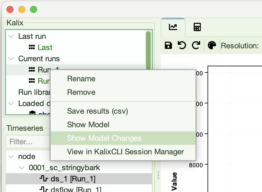
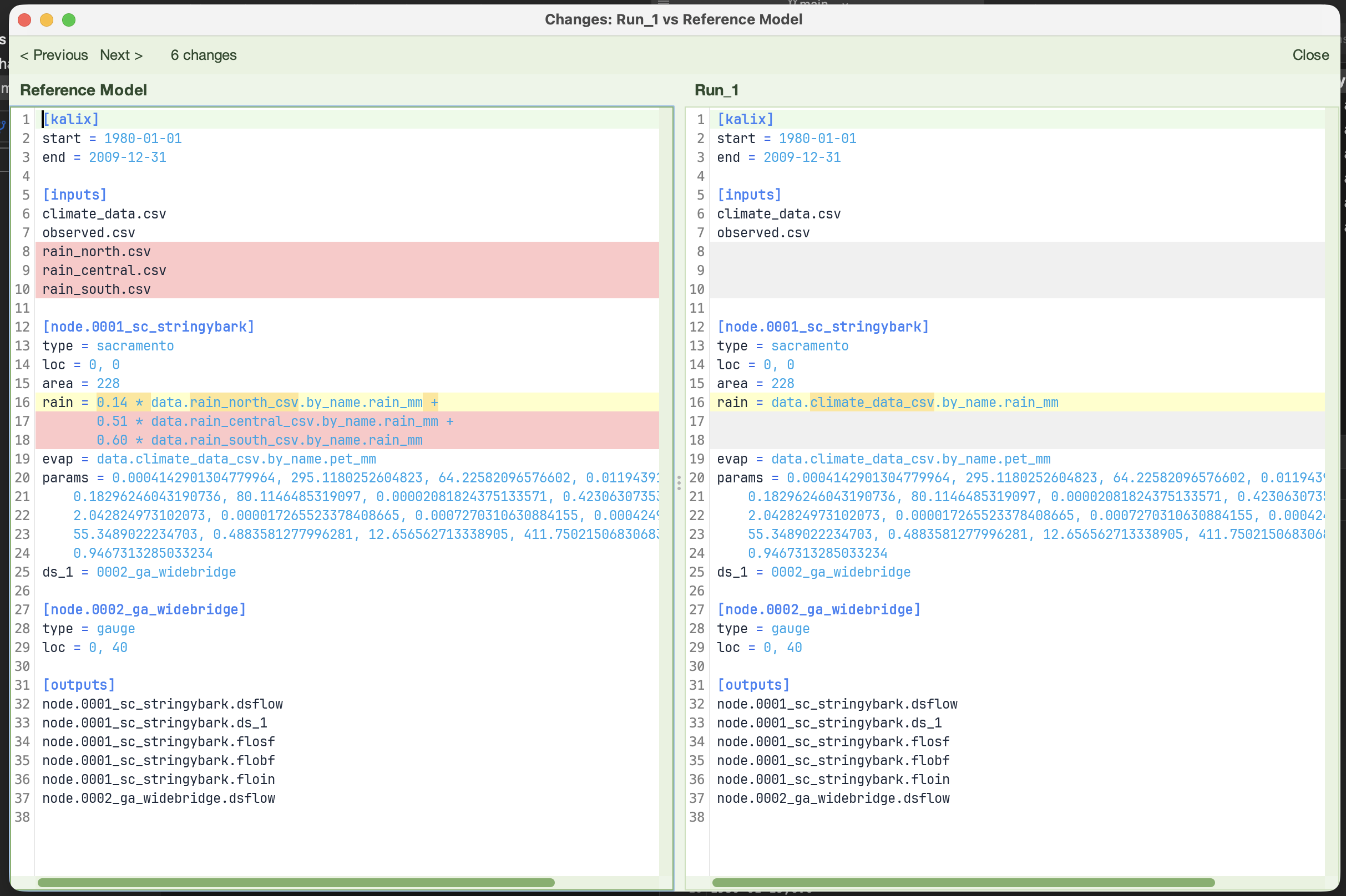
You can also inspect the model-file changes that drove this difference. Right-click the Tutorial 1 run in the Run Manager and choose "Show Model Changes". This opens a side-by-side diff between the model that produced the selected run (Tutorial 1's stringybark_sacramento.ini) and the model currently loaded in the editor (Tutorial 2's stringybark_expressions.ini). You should see two regions of difference:
-
The
[data]section, with the three new station files added -
The
rain = …line, with the single-column reference replaced by the three-line weighted expression
The overlay above shows you how the simulated flow changed; "Show Model Changes" shows you what changed in the model file to make that happen.
What to try next
Small experiments. Each one only changes the rain or evap expression.
-
Equal weights — try
(data.rain_north_csv.by_name.rain_mm + data.rain_central_csv.by_name.rain_mm + data.rain_south_csv.by_name.rain_mm) / 3. This is the plain average of the three stations. Compare with the weighted version in Run Manager. -
Drop a station — what if
rain_southdata was unavailable? Replace its term with0.60 * data.rain_central_csv.by_name.rain_mmto substitute the central station's series. How does that change the modelled flow? -
Scale PET for a warmer scenario — change
evap = data.climate_data_csv.by_name.pet_mmtoevap = 1.15 * data.climate_data_csv.by_name.pet_mm(15% more evaporative demand). Compare in Run Manager. -
Use parentheses to group an expression — wrap the weighted sum in parentheses and multiply by
1.1to scale the combined rainfall up by 10%:rain = 1.1 * (0.14 * data.rain_north_csv.by_name.rain_mm + 0.51 * data.rain_central_csv.by_name.rain_mm + 0.60 * data.rain_south_csv.by_name.rain_mm). Useful when you want to layer a climate-change factor over an existing combination of inputs.
Where to go from here
-
Tutorial 3 — Relative paths and trailhead paths — your input files live in a folder. What happens when you move the model? How do you build models that travel cleanly with their data?
-
Tutorial 4 — Running Kalix from the commandline — leave the IDE behind and drive Kalix from a terminal — the foundation for scripting and batch runs.