Tutorial 5 — Running Kalix from Python
Tutorial 5 of the Kalix tutorial series. You'll drive a Kalix simulation directly from Python using the kalix package, read the outputs as pandas DataFrames, and plot them. Expected time: about 20 minutes.
What you'll build
A Jupyter notebook that sits next to your model file and:
-
Runs the simulation with one line:
kalix.simulate(...) -
Reads the output into a pandas DataFrame
-
Plots simulated vs observed flow
-
(Bonus) Switches the output to Kalix's native Pixie format for faster, smaller files
This is the foundation for any analysis, scripting, or notebook-driven workflow built on top of Kalix.
Prerequisites
-
Kalix software and the Tutorial files — refer to Tutorial 1 — Your first model.
-
Tutorial 3 complete (or its concepts) — see Tutorial 3 — Relative paths and trailhead paths. We start from a project laid out the same way: shared
data/with a model inmodels/baseline/. -
Python 3.9 or newer with Jupyter installed.
-
Tutorial files — download the
005/folder from the KalixTutorials repository. The repo also ships a fully-workedanalysis.ipynbif you'd rather skim than type along.
Project layout
005/
├── data/
│   ├── climate_data.csv
│   ├── observed.csv
│   ├── rain_north.csv
│   ├── rain_central.csv
│   └── rain_south.csv
└── models/
    └── baseline/
        ├── stringybark.ini     ← the model (uses trailhead paths)
        └── analysis.ipynb      ← the notebook we'll write
The notebook sits next to the model file. That's deliberate — keep your scripts and analysis alongside the artefact they operate on so relative paths stay simple.
Step 1 — Install the kalix package
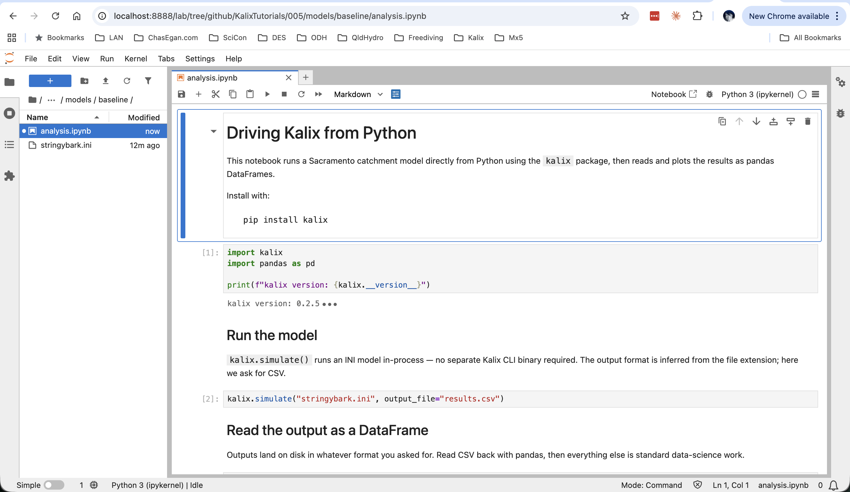
This installs the kalix Python package, which bundles the Kalix simulation engine as a native extension. You don't need to install the Kalix CLI separately — the engine runs in-process from Python.
Verify it works:
Step 2 — Open a notebook in the model folder
This launches Jupyter Lab with models/baseline/ as its working directory — so any relative paths from the notebook resolve cleanly against the model.
Create a new notebook and call it analysis.ipynb.
Step 3 — Run the model from Python
Imports and a single call:
That's it. kalix.simulate() runs the INI model in-process and writes the requested outputs to results.csv. The format is inferred from the file extension.
Step 4 — Read the output and plot it
The CSV that Kalix writes is just a normal time-indexed file. Pandas reads it directly:
You should see one column per output series declared in the model's [outputs] block — six columns in our case (the Sacramento total flow, its three runoff components, the link flow, and the gauge total flow).
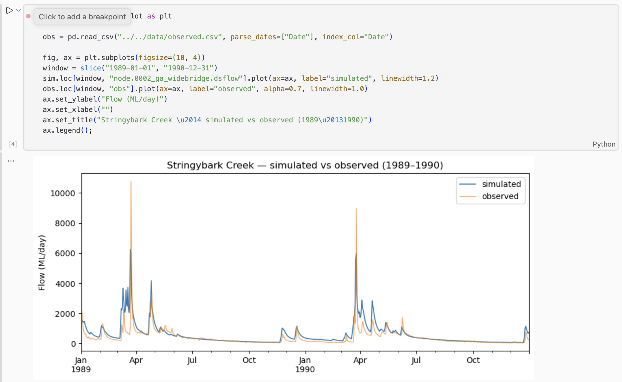
Now overlay simulated against observed:
import matplotlib.pyplot as plt

obs = pd.read_csv("../../data/observed.csv", parse_dates=["Date"], index_col="Date")

fig, ax = plt.subplots(figsize=(10, 4))
window = slice("1989-01-01", "1990-12-31")
sim.loc[window, "node.0002_ga_widebridge.dsflow"].plot(ax=ax, label="simulated", linewidth=1.2)
obs.loc[window, "obs"].plot(ax=ax, label="observed", alpha=0.7, linewidth=1.0)
ax.set_ylabel("Flow (ML/day)")
ax.set_title("Stringybark Creek — simulated vs observed (1989–1990)")
ax.legend();
Step 5 (bonus) — Pixie format
Kalix's native output format is Pixie — Gorilla-compressed timeseries written as a .pxt / .pxb pair. It's much smaller and faster to read than CSV for big runs (think: many nodes over multi-decade simulations). For this little 30-year, 6-output example the win isn't visible, but the syntax is identical and worth knowing.
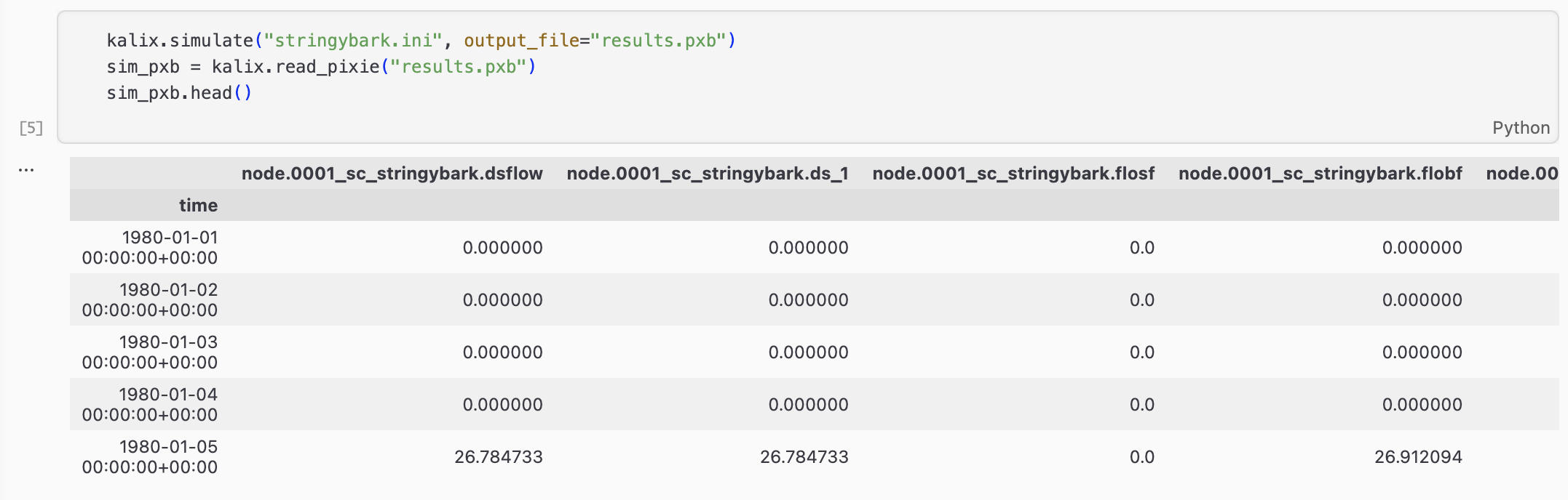
Switch the output by giving the simulator a .pxb extension:
Read it back with kalix.read_pixie():
The DataFrame has the same shape as the CSV version, but the index is now a tz-aware UTC DatetimeIndex named "time". From there all the standard pandas + matplotlib tools work the same way.
What to try next
-
Add a mass-balance report — pass
mass_balance="mbal.txt"tokalix.simulate(...)to write a plain-text report of inflows, outflows, and storage changes alongside the timeseries output. -
Loop over scenarios — write a Python loop that varies a scale factor on the rainfall expression, runs each scenario, and stacks the resulting DataFrames into a single multi-column DataFrame for comparison.
-
Round-trip your own data — use
kalix.write_pixie(path, df)to save any pandas DataFrame (with a UTCDatetimeIndex) into Pixie format. Useful for sharing pre-processed inputs across models.
Where to go from here
- Tutorial 4 — Running Kalix from the commandline — drive Kalix from a terminal instead of Python. Complementary skill for batch runs and CI pipelines.
The kalix Python package lives on PyPI: pypi.org/project/kalix. Current functionality and API are documented in the package README.